


How building automation impacts health, efficiency, and indoor air quality in hospitals
How does building automation ensure hospitals are safe, secure, comfortable environments for everyone?


The mechanical systems of a modern facility are often complex, expensive, and can consume significant energy. Improperly controlled these systems waste natural resources and fail to moderate the built environment. These same systems though can be harnessed by the hands of a capable automation professional just as a landscape can appear from beneath the brush strokes of an artist or a marionette can dance at the fingers of a puppeteer. To excel at their trade, the technician, artist, and performer must each exhibit understanding, knowledge, and skill; the skill manifested by a deft touch. Operational optimization of a complex mechanical system to deliver precise control while conserving resources requires this composite expertise. A deft touch with control loops empowers proper application and is a crucial technique for an effective automation professional, analogous to the subtle twist of an artist’s wrist or twitch of a performer’s finger.
The previous installment of insight provided a basic introduction to control loop theory, an overview of the action, proportional, integral, and derivative terms of a control loop, and how they are used by a MACH-System™ Loop object. In review, proportional, integral, and derivative are three independent corrective terms of a control loop. Proportional correction responds in proportion to error, or deviation from setpoint. Integral correction responds to offset, or error over time. Derivative correction responds to rate of change.
Imagine a holding tank that must maintain 100 units of water. If 25 units are drained, the tank holds 75 units. 25 units must be added to the tank to restore it to the desired volume of 100 units. This is a proportional response: 25 units are drained so 25 units are filled. Now imagine that the 25 units have been drained from the tank; however, this time, the drain valve remains open; allowing 25 units per minute to be released from the tank. Adding a proportional amount of water, 25 units per minute, will not restore the tank to 100 units, it will only prevent the tank from being drained. This proportional-only response will prevent greater error but will result in offset, or a sustained error over time. Slowly, incrementally, opening the fill valve more-and-more to add an ever-increasing volume of water (e.g., 26, then 27, then 28 units per minute) will eventually overcome the loss of 25 units per minute and will begin to fill the tank. This accumulated correction to the offset is an integral response. If a derivative response were implemented, it would open/close the fill valve whenever the water level changed in proportion to the rate of change; but, would have no effect when the water level is stable (regardless of error or offset). Since this control loop is adding water in response to a negative error (when the input is below the setpoint) it would be considered a reverse-acting control loop.
Before further consideration of how control loops are used, it is important to understand two remaining terms of the MACH-System Loop object.
Bias is a constant offset added to the corrective action of a control loop term when defining the composite control loop output. Bias is sometimes referred to as the null, or default value, for proportional-only control loops as it represents the output of a proportional loop when the input is at setpoint. Unlike proportional, integral, and derivative, the bias term is not automatically calculated by the control loop. A static bias value is often defined when tuning the loop. In advance applications, the bias can be modified dynamically and assigned programmatically.
In the MACH-System, the bias term corresponds to the Loop output range of 0-100 percent. When calculating the output of a Loop, the bias value is added to the proportional output (and the derivative output when used); then the sum is limited between 0-100 percent. For example:
|
Bias |
Proportional Output |
Loop Output |
||
|
50% |
+ |
0% |
= |
50% |
|
50% |
+ |
50% |
= |
100% |
|
50% |
+ |
100% |
= |
100% |
|
50% |
+ |
-50% |
= |
0% |
Table 1: Sample loop output calculations including bias and proportional output.
When using a biased control loop, negative corrective action is required to result in a loop output less than the bias (for instance 0 percent). A negative term (e.g., proportional or integral) output results from overshoot: negative error in a direct-acting loop or positive error in a reverse acting loop. Consider a direct-acting, proportional control loop with a 4˚ proportional band, a bias of 50 percent, and a setpoint of 22˚C:
|
Input |
Setpoint |
Error |
Proportional Output |
Bias |
Loop Output |
||||
|
22°C |
- |
22°C |
= |
0°C |
0% |
+ |
50% |
= |
50% |
|
24°C |
- |
22°C |
= |
+2°C |
50% |
+ |
50% |
= |
100% |
|
20°C |
- |
22°C |
= |
-2°C |
-50% |
+ |
50% |
= |
0% |
Table 2: Direct-acting proportional (4° proportional band) controls loop with 50 percent bias.
This is an example of a control loop that is biased in favor of cooling. Even when the space temperature is at the setpoint, the bias results in a corrective output from the control loop. Only when the space temperature falls below the setpoint is corrective action reduced and ultimately eliminated.
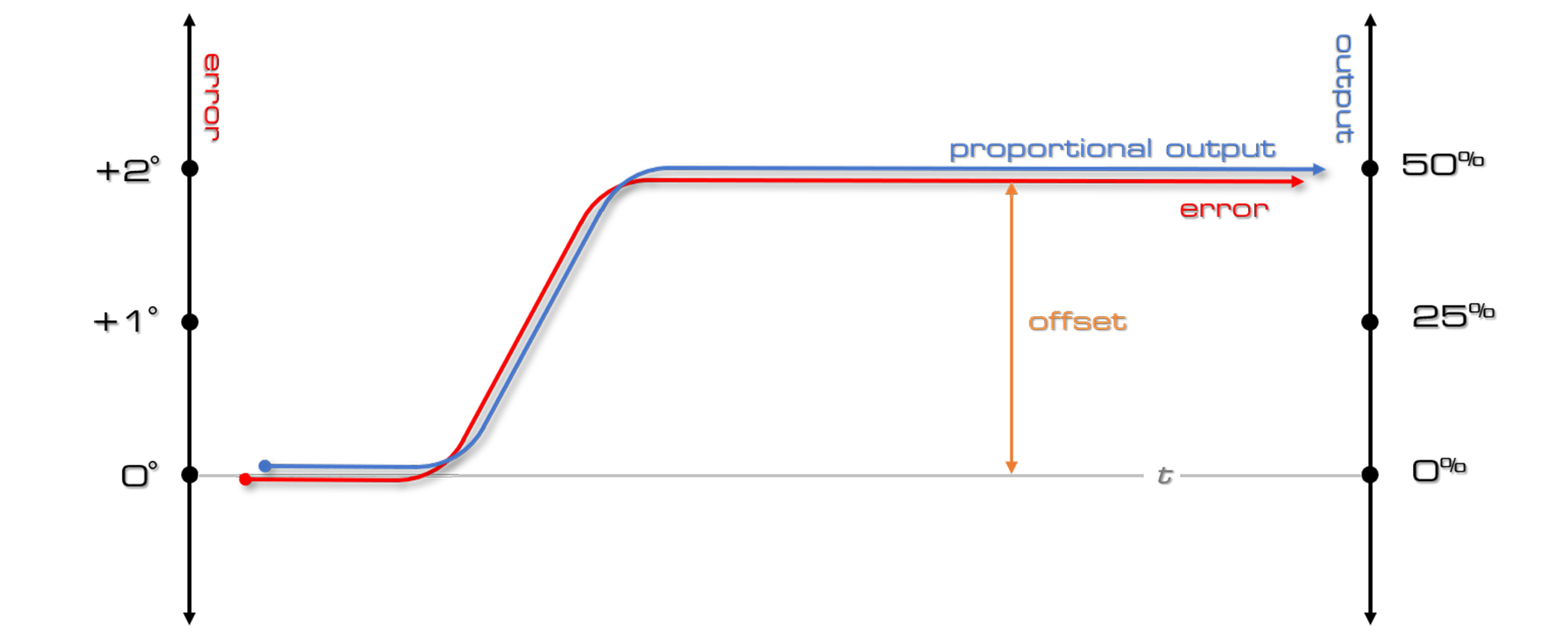
For stable applications, bias can be added to overcome the sustained offset typical in proportional-only control. Consider the example described in introduction to Table 2. Imagine that an output of 50 percent is sufficient to maintain a 2°C error. If the input does not change, the error will not change. If the error does not change, the proportional output will not change. While this is stable control, it also represents a persistent 2°C offset, or error over time. Proportional control will not attempt to eliminate this offset.
Figure 1: Proportional-only output resulting in offset (error over time).
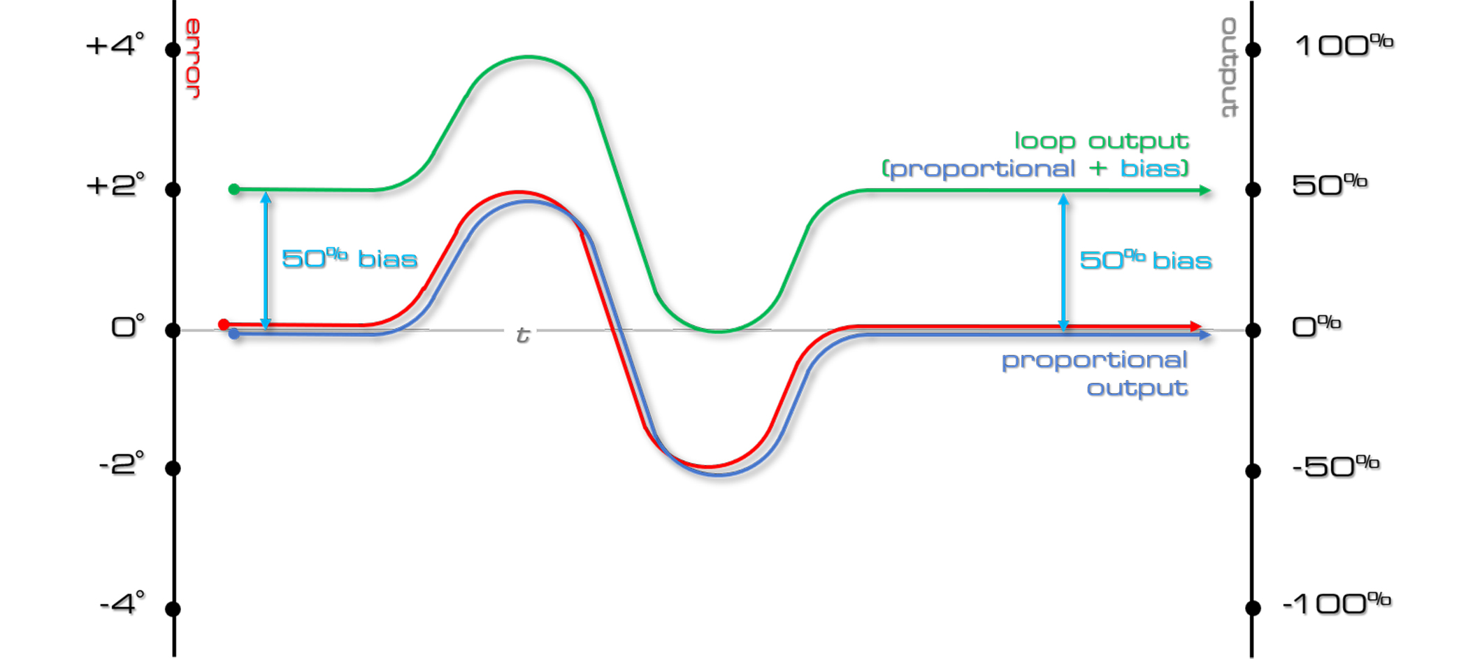
When the input is at setpoint, a bias of 50 percent would complement the proportional output to result in 50 percent correction (50 percent bias + 0 percent proportional output = 50 percent loop output). In normal conditions, this bias might be sufficient to eliminate the offset. As the error fluctuates, proportional control added to the bias will provide a normal proportional control response. As the error rises from 0˚C to 2˚C above setpoint the proportional output added to the bias will result in a Loop output modulation from 50 percent to 100 percent (where the Loop output is inherently limited). Conversely, when the error falls from 0˚C to 2˚C below setpoint the proportional output subtracted from to the bias will result in a Loop output modulation from 50 percent to 0 percent (where the Loop output is again inherently limited).
Figure 2: Composite control loop output: proportional output + bias (50 percent).
In this way, bias is an important term for loops in control of applications where an input cannot be maintained with a 0 percent output command. For example, even when the input is at setpoint, variable speed fans or pumps must operate at a speed greater than 0 percent to maintain pressure or flow in a dynamic system.
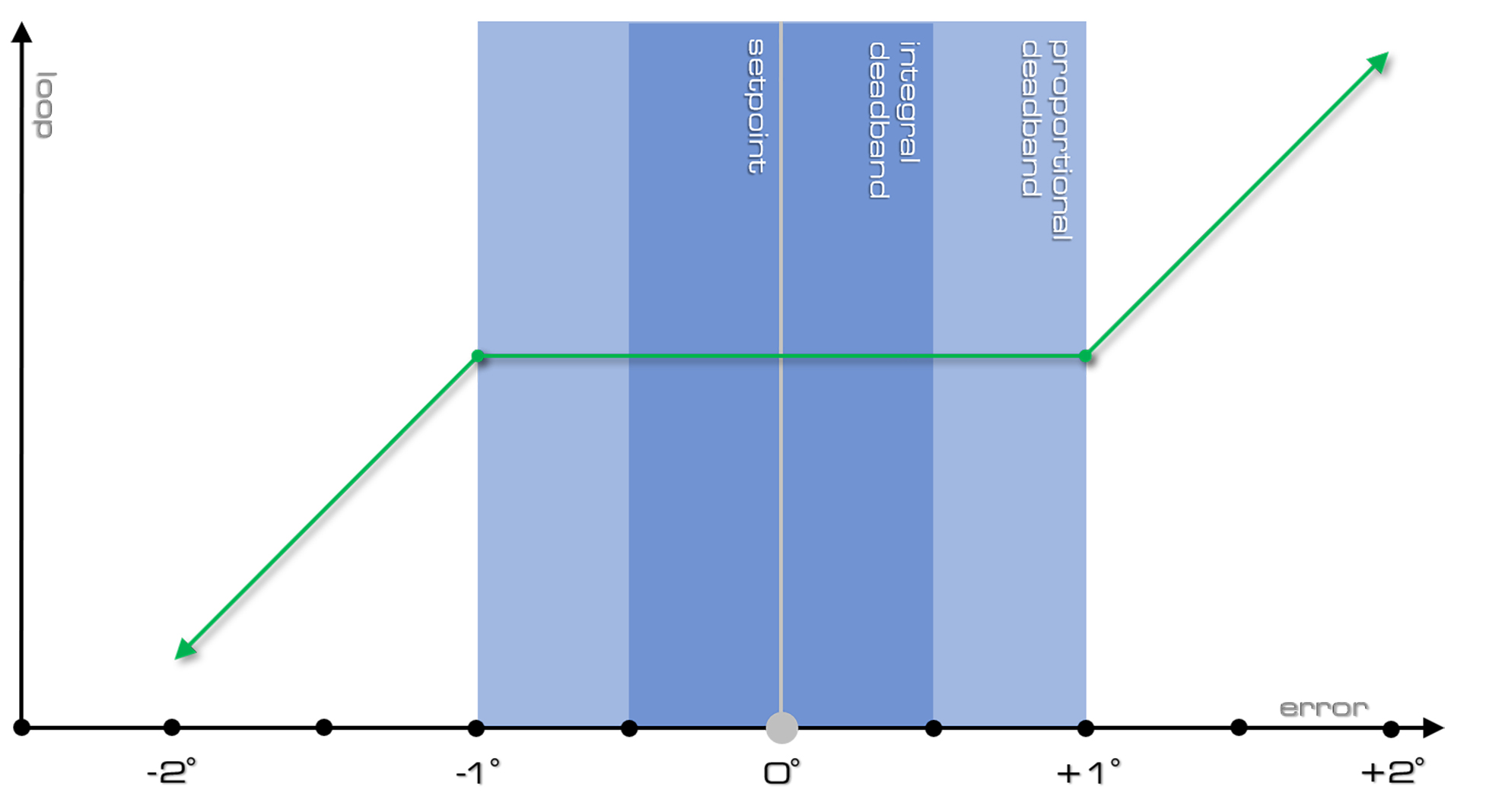
Deadband is a term in a MACH-System control loop that can be used to pause correction when the input nears the setpoint. The deadband is expressed in the same units as the input, setpoint, and proportional band. The deadband value is automatically divided and applied evenly above and below the setpoint.
Figure 3: Loop output illustrated with a 2° deadband applied evenly above and below the setpoint.
Proportional correction is paused when the input is within the configured deadband. Integral correction is paused when the input is within half the configured deadband. This means that with a 2˚F deadband and a 72˚F setpoint, proportional correction is paused between 71˚F to 73˚F, and integral correction is paused between 71.5˚F to 72.5˚F.
The terms of a control loop can be used individually or in cooperation to provide an appropriate corrective control response to the dynamic processes in facility automation applications.
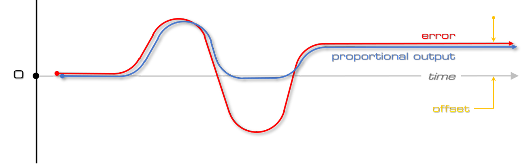
A proportional control loop provides a corrective control response based upon error.
Figure 4: Proportional-only control loop output (limited 0-100 percent) over time, in response to error.
As a proportional response is dependent on deviation, proportional-only loops often result in sustained offset. If the offset is prohibitive, another term, such as integral and/or bias, can be added.
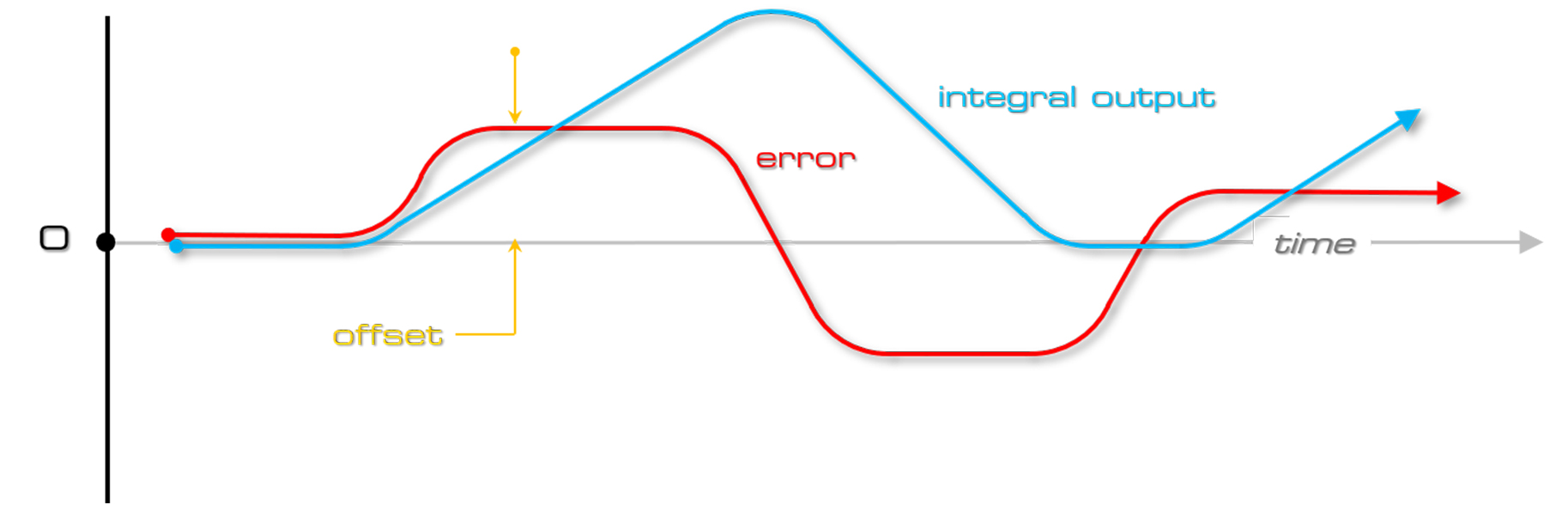
An integral control loop provides a corrective control response based upon offset, error over time. The integral response accumulates gradually based upon the error and the integral reset time.
Figure 5: Integral-only control loop output, or reset control (limited 0-100 percent), over time in response to offset.
As an integral term continues to provide correction to offset until there is no error, it can result in overshoot. Properly tuned, the magnitude of the overshoot should lessen in subsequent cycles.
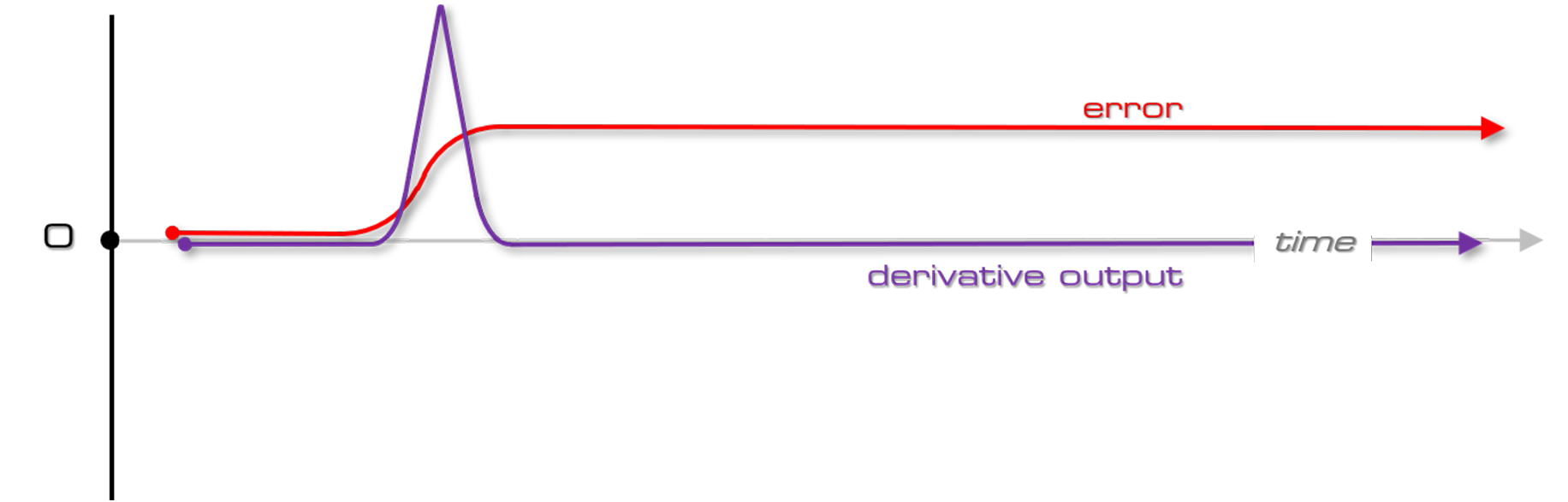
A derivative control loop provides a corrective control response based upon rate of change. When the error is stable, zero derivative correction is provided. A derivative term can be used as an anticipator to counteract change when very little error is acceptable and the corrective action (output) may have an immediate and substantive effect on the process variable (input). Derivative is calculated in minutes (0-2). It anticipates, based on the present rate of change, where the error will be in the future (based upon the configured derivative rate), and immediately corrects with the magnitude of that anticipated error. For instance, if the setpoint was changed by 1˚ since the last execution, the rate of change is 1˚ per second. With a derivative rate of 1 minute, the output would immediately counteract an anticipated change of 60˚ (1˚/s x 60 seconds) with an output increase of 60 percent. One second later, with no further change in error, since neither the input nor the setpoint has changed, the derivative output returns to 0 percent.
Figure 6: Derivative-only control loop output (limited 0-100 percent) over time, in response to error rate of change.
When used, derivative is often combined with another control loop method and is one term of Proportional Integral Derivative (PID) control loops. The nature of the derivative term can make it difficult to properly tune and inappropriate for many comfort control applications where control responses seldom have an immediate and substantive effect on the process variable.
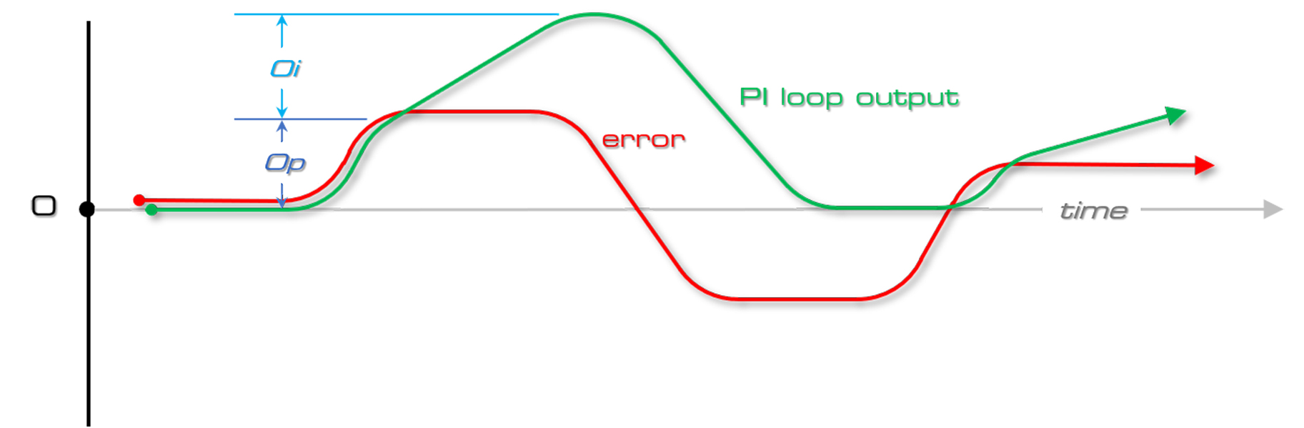
Proportional Integral, or PI, control combines the actions of the Proportional and Integral terms. Proportional correction is provided immediately in proportion to the deviation from setpoint. The integral correction accumulates gradually to reduce the offset. This type of control is commonly applied where proportional control alone would result in an unacceptable offset.
Figure 7: Proportional (Op) Integral (Oi) control loop (PI) output over time, in response to error and offset.
A majority of comfort control, HVAC applications are satisfied using PI control.
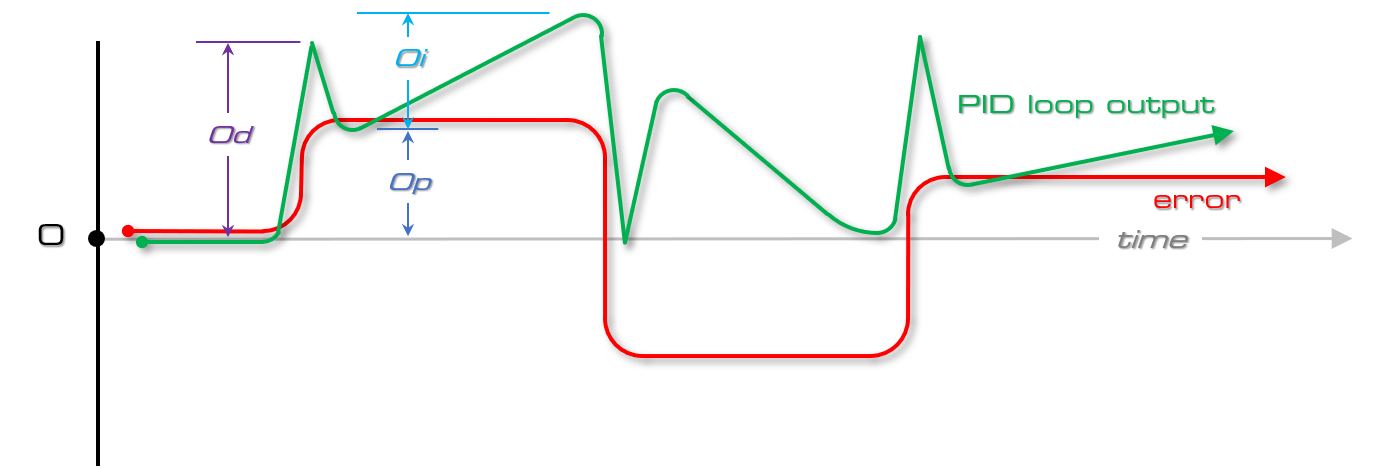
Proportional Integral Derivative (PID) control combines the actions of the Proportional, Integral, and Derivative terms. The derivative component is first applied to act as an anticipator and acts to slow the rate of change. Proportional correction is provided immediately in proportion to the deviation from setpoint. Finally, integral correction accumulates gradually to reduce the offset.
Figure 8: Proportional (Op) Integral (Oi) Derivative (Od) control loop (PID) output over time, in response to rate of change, error, and offset.
This type of control is used when there are sudden changes to the measured variable, precise control is critical, and the output has an immediate and substantive effect on the input.
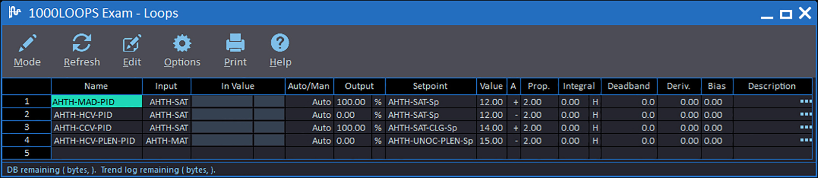
A MACH-System Loop is configured using the Loops worksheet in RC-Studio®.
Figure 9: RC-Studio 3 LOOPS worksheet populated with proportional-only control loops.
All the information necessary to properly tune the Loop object is presented in the worksheet.
|
Column |
Description |
|
Name |
32-character name for the Loop. |
|
Input |
Object to be referenced as the process variable. This measurement, or feedback, drives the corrective actions of the control loop and is controlled by a closed-loop. |
|
In Value |
The present value of the input object. |
|
Auto/Man |
In Auto, the control loop output is automatically calculated. In Manual, the control loop output is not automatically calculated and may be indexed by the operator. |
|
Output |
The composite control loop output; the sum of Op + Oi + Od + Ob limited to 0-100 percent. |
|
Setpoint |
Object to be referenced as the setpoint for the control loop. Input - Setpoint = Error. |
|
Value |
The present value of the setpoint object. |
|
A |
Action of the control loop; direct-acting (+), or reverse-acting (-). |
|
Prop. |
Control loop proportional band. Expressed using the same units as the input, setpoint, and deadband. The amount of deviation that results in 100 percent proportional output (Op). |
|
Integral |
Control loop integral reset time. This defines the number times per minute (M) or hour (H) that the magnitude of the error is added-to or subtracted from the integral output (Oi). |
|
Deadband |
Range surrounding the setpoint within which proportional and integral correction is inactive. |
|
Deriv. |
Control loop derivative rate. Derivatives are expressed from 0.00–2.00 minutes; a higher value causes a larger output to oppose the changing input. |
|
Bias |
Control loop constant output. The value of the loop output for a purely proportional loop, when the Input equals the Setpoint. Expressed in units of the output 0-100 percent. |
|
Description |
255-character description. |
Table 3: RC-Studio LOOPS worksheet columns.
The MACH-System Loop is automatically calculated as follows:
1. The sum of Op + Od + Ob is limited to 0–100.
2. Oi is added to the result of Step 1.
3. The result of Step 2 (the Loop output) is limited to 0–100.
4. Oi is adjusted (for the next scan) by the amount the output was limited in Step 3 (e.g., if the output was reduced from 103 to 100 in step 3, the accumulated Oi will be reduced by 3 percent prior to the calculation in the subsequent execution).
Where:
When the Auto/Man parameter is set to Auto, MACH-System Loops calculate the composite control loop output once per second. The proportional, integral, and derivative outputs are calculated each execution:
This incremental integral correction results in a smoother integral output rather than a stepped output resulting from adding the total correction at the configured integral reset time.
Static configuration of the control loop parameters can be set using the LOOPS worksheet in RC-Studio. Dynamic configuration for advanced applications is possible using Control-BASIC. Each control loop parameter (setpoint, action, proportional band, integral reset, derivative rate, bias, and deadband) can be read-from and written-to using standard BACnet properties as described in the BACnet Properties forum available from the Reliable Controls website Support Center eForum. The Control-BASIC syntax library also includes functions to dynamically define the control loop gains for proportional band (CONPROP), integral reset (CONRESET), and derivative rate (CONRATE). Applications and examples of dynamic control loop adjustment are provided in the Control-BASIC Manual 2nd Edition, also available from the Support Center.
In addition to modifying the control loop parameters, the basic execution of MACH-System control loops can also be directly manipulated by Control-BASIC programs.
Using the STOP statement (e.g., STOP LOOP1) has the following effects:
• The Loop is placed in Manual.
• The Loop is prevented from calculating.
• The Loop output remains persistent at the last calculated value.
Stopping a Loop in the MACH-System will prevent further execution; however, it will not reset the output to 0%. In effect, the Loop object is simply paused. The output value remains static so long as the Loop remains in Manual. This does not pose a functional issue. The output of the loop is assigned to a physical output in Control-BASIC, so the physical output can be zeroed or otherwise commanded for off-cycles programmatically. The proportional output is always instantaneous, so there is no need for it to be zeroed; e.g. even if the off-cycle proportional output was zero, the first execution the total effective proportional output would be calculated and applied. Only the integral output is accumulative, and it can easily be reset on demand by using the START statement.
Using the START statement (e.g., START LOOP1) has the following effects:
• The Loop is returned to Auto.
• The integral corrective action is reset to 0 percent.
• The Loop calculates normally on each execution.
Starting a Loop in the MACH-System effectively returns the Loop object to Auto with one important additional feature: the accumulated integral corrective action is reset to 0 percent. This can be beneficial for resetting any accumulated integral wind-up at the beginning of a cycle. Caution must be taken to conditionally apply START to a Loop only as necessary. As START resets the integral corrective action each time it is executed, if the Loop is started every scan of a normal equipment cycle, it will never be able to accumulate an appropriate integral response. A Loop can be started even if it has never been stopped; i.e., there is no requirement to STOP a Loop to reset the integral using START. Proper deployment examples include:
10 IF+ MODE-OCC THEN START LOOP1 : REM ** Reset integral on transition to occupied.
10 IF+ CLG-ENA THEN START AH01-LOOP-CLG : REM ** Reset integral when cooling is enabled.
10 IF NOT MODE-OCC THEN START LOOP1 : REM ** Prevent integral during unoccupied.
Using the START statement is a simple an effective method for resetting the integral windup at the beginning of an active cycle, or preventing it during an inactive cycle.
Finally, it is also possible to write a value to a Loop object; for example, LOOP1 = 22. This syntax does not index the output of the Loop; rather, it is used assign the setpoint of the loop. If it is essential for a control loop output to be 0 percent during an inactive cycle, this can be used to zero the proportional output:
10 IF NOT MODE-OCC THEN ZN10-LOOP-CLG = ZN10-RMT
Assigning the value of the control loop input to the loop as the setpoint results in zero error which will returns zero proportional output. Of course, if integral and/or bias are used, these terms would have to be zeroed as well.
Deft denotes skillful, quick, adapt in action or thought. A deft touch in the application of control loops is a defining trait of an automation professional. Even when it comes naturally, skillfully manipulating a paint brush, a puppet, or a facility requires understanding, knowledge, skill, and practice. Fortunately, all of these lie within our grasp, we need only cultivate the desire.
The next installment of insight will conclude the discussion of MACH-System control loops with best practices for proper control loop tuning.

How does building automation ensure hospitals are safe, secure, comfortable environments for everyone?

Learn when and why MS/TP communication is helpful in building automation systems.

From the moment you park your car at a hockey arena, your comfort and safety are enhanced through a building automation system. Here’s how.

Building automation systems can make buildings truly intelligent, reducing their carbon footprint and saving money. Learn how.

Ever wonder how a building automation system ensures safety and accuracy in lab work?

Museums—and their building automation systems—play an important role in preserving the preserved. Learn how.
When you see a doctor or personal trainer, you benefit from their knowledge and experience. In the same way, a building automation system should provide all the tools you need to maintain your buildings in optimal health.

What are you doing to mitigate the transmission of viruses indoors? Learn what measures you can take and how your smart building provides more information and control for IAQ concerns.