An orchestra is an instrumental ensemble comprised of perhaps one hundred or more musicians playing instruments from different families together, in performance of a composition. An orchestra is often lead by a conductor, whom is responsible for the rhythm and tempo of the music played by the musicians; but more than that, the conductor’s trained, critical ear and highly-refined expertise play a significant role in the interpretation of the composition into a poignant, aesthetic experience.

The mechanical systems of modern facilities are comprised of numerous and varied components and sub-systems. Like a conductor, a skilled-automation professional can use understanding, critical observation, and highly-refined expertise to synchronize these systems into a concerted ensemble. One of the nuances that should be finely manipulated in a facility are the control loops that guide the operation of mechanical equipment and systems.

The previous installments of insight provided a basic introduction to control loop theory and to the terms used in MACH-System control loops. The purpose of a control loop is to provide automatic control that is responsive to change and results in a stable process. For optimal performance, each term of the control loop must be properly tuned to provide:

• Appropriate correction in response to error; as determined by the proportional band;
• Proper accumulation of correction to eliminate offset; as determined by the integral reset; and
• An ideal rate of correction to counteract the changing input; as determined by the derivative rate (where required) .

Each application is unique. Even typical applications within a common system can have subtle differences. These differences in the physical characteristics of the equipment, process, and environment for each application must be considered to provide a system that is both responsive to change while providing stable control. This is the primary reason for the Reliable Controls Best Practice Programming Rule that every analog output application should have a dedicated control loop. While it is possible, and can be tempting, to control an air handling system with a single temperature control loop, heating and cooling coils seldom have the same capacity or control characteristics, and cooling with a chilled water or a direct expansion coil is seldom identical to cooling with outdoor air. Each analog application should be properly tuned to account for the subtle variances in physical characteristics.

The term tuning implies action; specifically to tune-the act of adjusting or balancing a musical instrument to a proper pitch, or a process to achieve proper performance. Just as a musician cannot walk up to a stringed instrument, turn the tuning pegs, and play a beautiful piece of music without listening to the sounds of the instrument, an automation process cannot be properly tuned by setting-it-and-forgetting-it. Control loop tuning deserves appropriate consideration. Temptations to seek shortcuts are seldom effective. Fortunately, with just a little experience and focus, MACH-System control loops can be easily tuned.

Poor Control Loop Performance

Poor control loop performance resulting from improper tuning in comfort control applications can generally be categorized in one of three ways:

• OFFSET. Offset is characterized as error over time. An improperly tuned control loop can provide a stable process that fails to maintain the input at the setpoint. Sustained error makes it easy to identify a control loop with offset. A loop that exhibits sustained offset typically needs to be more aggressive.

• LEADING. A leading control loop is sometimes described as hunting, cycling, or oscillating. All these terms can be used to describe a control response that has excessive variance. It is sometimes referred to as leading because severe correction dramatically leads, or forces, the input. When there is error, a leading loop over-corrects, resulting in a significant output, and a rapid elimination of the error. As the error is reduced (and often overshoots the setpoint), the loop again over-corrects, and significantly reduces the correction, allowing error to quickly return. The output can be said to oscillate or cycle because it is unstable, continuously increasing and decreasing; resulting in a valve constantly opening and closing, or a motor continuously speeding-up and slowing-down. It is said to hunt, as the oscillation of the output results in an input that cannot find the setpoint. Leading loops are easily identified in a trend log with outputs and inputs that present in a sinusoidal wave, constant cycles up-and-down, typically with a short frequency. Leading loops need to be less aggressive.

• FOLLOWING. A following control loop is sometimes described as a lagging control loop. Just as the output of a leading control loop leads the input, the output of a following control loop follows the input. A following loop lags or responds too slowly to changes in the input. Following loops can be more difficult to identify than leading loops, but present similarly. Lagging loops will also exhibit in a trend log with outputs and inputs that present in a sinusoidal wave form; however, the frequency is generally longer. Following loops will typically not present with drastic cycling, but rather a sustained, ever-changing variance in the input and output. Following loops need to be more aggressive.

The aggression of a control loop can be used to describe the magnitude, accumulation, and rate with which it responds to changes in the process variable. A more aggressive control loop responds with greater correction to error more quickly. A less aggressive control loop responds with less correction to error more slowly. The aggression of each control loop term is tuned individually to achieve the ideal response.

Table 1: Control loop aggression configuration and results by term.

Control loops must be tuned to the physical characteristics of the equipment, process, and environment so that a change in the input is counteracted with an output that is appropriate to eliminate error without introducing process instability, excessive overshoot, and hunting.

Control Loop Tuning

Testing and tuning a control loop are performed by introducing a disturbance to an operational process. One of the preferred methods to create this disturbance is by changing the setpoint. A disturbance can also be introduced to the system by creating a natural error; for instance, by manually closing a chilled water valve and allowing the temperature to rise, or manually slowing a fan or pump and allowing the pressure to drop. In either case the process must be operationally, consistent with the design parameters.

Once the disturbance impacts the process, closely observe the response of the control loop and the corrective output. Proportional correction should cause a measured and immediate response to the error, and then integral reset will begin to slowly ramp the output further. Once the output begins to influence the process variable, the input will begin to change. Once the error begins to reduce, the control loop should guide the input back to setpoint.

There are many standard methods for tuning control loops. Some utilize rules of thumb while other use complex mathematical equations and software programs. The proper technique is the one that consistently results in control loops that are responsive to change while providing stable control. Consider one simple approach that has proven to be efficient and effective.

Control Loop Tuning: A Method

As the individual terms of a control loop respond individually, it is recommended to the tune them individually. Begin tuning with a proportional-only control loop. Set the integral reset, derivative rate, deadband, and bias to 0.

Proportional Band (Prop.)

The proportional band is tuned to achieve a stable response. Do not be concerned with error.

1. Start with a small proportional band that results in hunting.

2. The initial proportional band can be determined analogously (e.g., based upon experience with previous similar applications) or parametrically (e.g., based upon the maximum allowable deviation). In the absence of analogous or parametric data, simply start with a desired control variance (e.g., 1–2˚, 1 inwc., 250 Pa, etc.).

3. Observe the response of the control loop. Be sure to provide adequate time to evaluate the responsiveness of the loop before making changes.

4. Does the control loop cycle, or hunt? If the output of the loop and the process variable peak equally but oppositely (e.g., the loop output is at its highest point when the input is at its lowest point, or the loop output is at its lowest point when the input is at its highest point), the process is likely hunting due to an overly-aggressive proportional band. Increasing the proportional band will eliminate or reduce this oscillation.

5. If the loop hunts, increase the proportional band by 100% (e.g., increase from 2 to 4, 4 to 8, 8 to 16, etc.). Return to step 3.

6. If the loop lags, decrease the proportional band by 50% of the last change. For instance, if the last change was an increase from 16 to 32, and the loop is now lagging, decrease the proportional band to 24 (e.g., 32 - 16 = 16; 16 / 2 = 8; 32 - 8 = 24).

7. Observe the response of the control loop.

8. Does the control loop lag? If so, return to step 6.

9. If the control loop does not lag, does the control loop now cycle, or hunt?

10. If the control loop now hunts, increase the proportional band by 50 percent of the last change. For instance, if the last change was a decrease from 32 to 24, and the loop is now cycling, increase the proportional band to 28 (e.g., 32 - 24 = 8; 8 / 2 = 4; 24 + 4 = 28). Return to step 7.

11. Eventually the response of the loop will stabilize and neither lead nor lag the input. Changes to the setpoint or input will result in a corrective action that is appropriate to bring the input to a stable state (it may not eliminate the error), to control the input, promptly and without cycling.

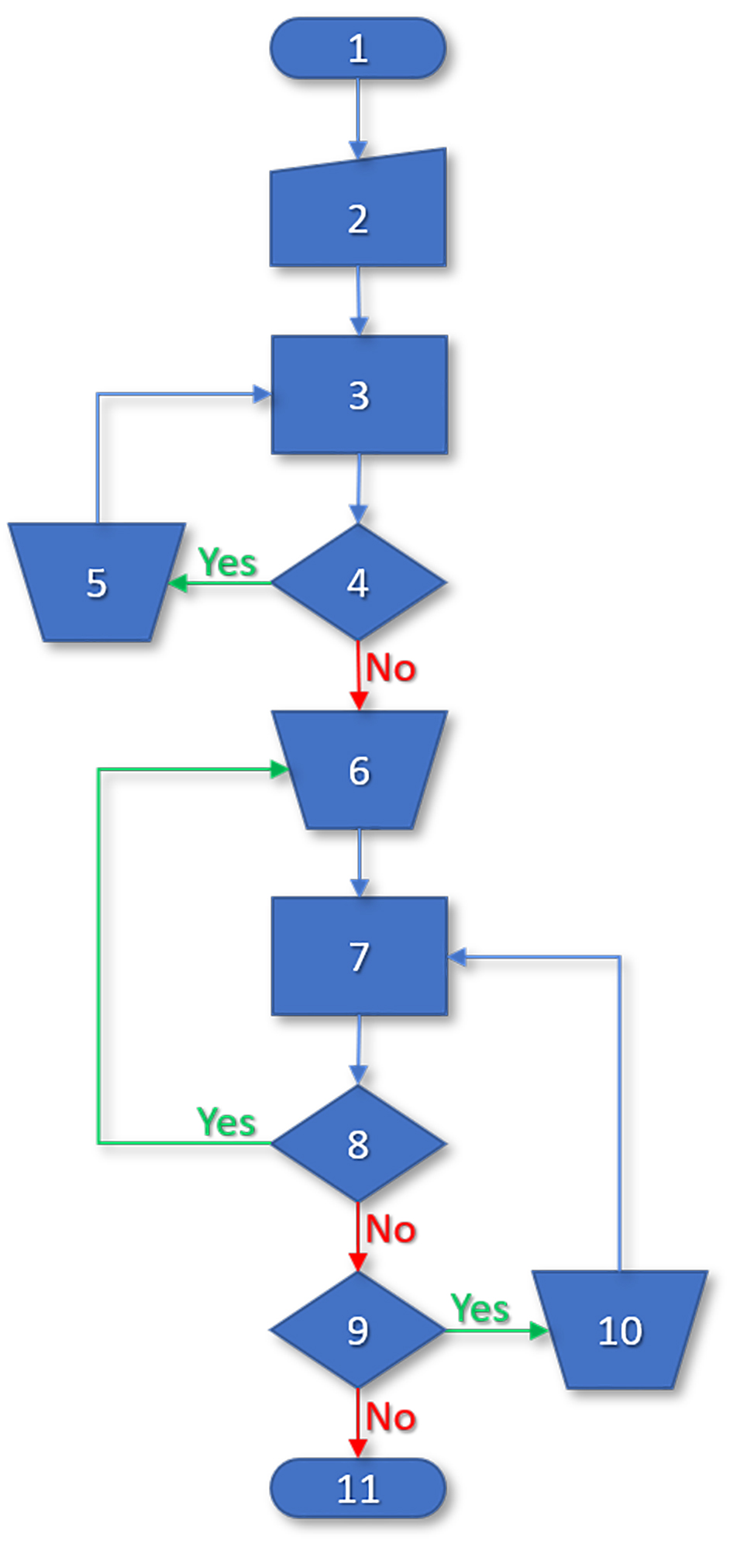
Figure 1: Proportional band tuning process flowchart.

This is an iterative cycle of observation and fine-tuning. Be sure to provide adequate time to evaluate the responsiveness of the loop following each iteration before making changes.

In many applications, particularly with a diverse design range, it is likely that a proportional band that results in a stable response will also result in an undesirable offset. Once the proportional response is properly tuned, integral reset can be added to the loop to eliminate this offset.

Integral Reset (Integral)

The integral reset must be carefully tuned to eliminate the offset without introducing excessing overshoot or cycling to the process.

1. Start with a slow integral reset, configured as repeats per Hour (H).

2. The initial integral reset can be determined analogously or parametrically. In the absence of analogous or parametric data, consider 4/H (15-minute reset), 6/H (10-minute reset), or 12/H (5-minute reset) integral reset times.

3. Observe the response of the control loop. Be sure to provide adequate time to evaluate the responsiveness of the loop before making changes.

4. Does the control loop eliminate error quickly enough to be appropriate for the application?

5. If the elimination of error is too slow for the application, increase the integral reset by 100 percent (e.g., increase from 6 to 12, 12 to 24, 24 to 48, etc.). Return to step 3.

6. When the loop eliminates error, it will result in some overshoot (e.g., the input pushed below the setpoint in a direct-acting loop or the input pushed above the setpoint in a reverse-acting loop). Slight overshoot that diminishes over time is expected. Significant overshoot will result in hunting.

The PI control loop response should transition from increasing correction to decreasing correction before the input reaches the setpoint. If correction is still increasing, if the corrective output peaks, when or after the input reaches the setpoint, then the loop is likely to result in undesirable overshoot and cycling because of too much integral reset. Reducing the integral reset will eliminate or reduce this oscillation.

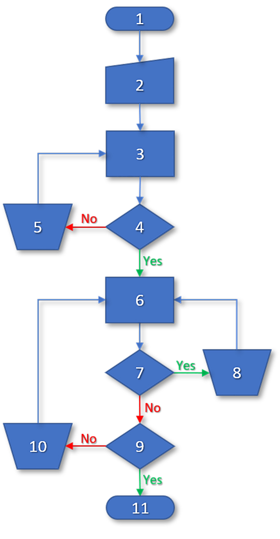
Figure 2: Integral reset tuning process flowchart.

Observe the response of the control loop, particularly the magnitude of the overshoot and the time required to bring the correction to zero. Be sure to provide adequate time to evaluate the responsiveness of the loop before making changes.

7. Does the loop overshoot the setpoint significantly, causing the loop to cycle or hunt?

8. If the control loop hunts, decrease the integral reset by 50 percent of the last change. For instance, if the last change was an increase from 24 to 48, and the loop is now cycling, decrease the integral reset to 36 (e.g., 48 - 24 = 24; 24 / 2 = 12; 48 - 12 = 36). Return to step 6.

9. When the loop does not cycle, does it eliminate error quickly enough to be appropriate to the application?

10. If the elimination of error is too slow for the application, increase the integral reset by 50 percent of the last change. For instance, if the last change was a decrease from 48 to 36, and the response is now too slow, increase the integral reset to 42 (e.g., 48 - 36 = 12; 12 / 2 = 6; 36 + 6 = 42). Return to step 6.

11. Eventually the loop will provide an output that is appropriate to eliminate error without introducing process instability, excessive overshoot, and hunting.

An integral reset of 60/H is equal to 1/M. If an integral reset of 60/H or greater is required, consider changing the integral reset configuration from Hours (H) to Minutes (M).

After the proportional integral (PI) loop has been tuned, additional terms can be added. For most HVAC comfort control applications, a properly tuned PI loop can provide stable, highly accurate and precise control.

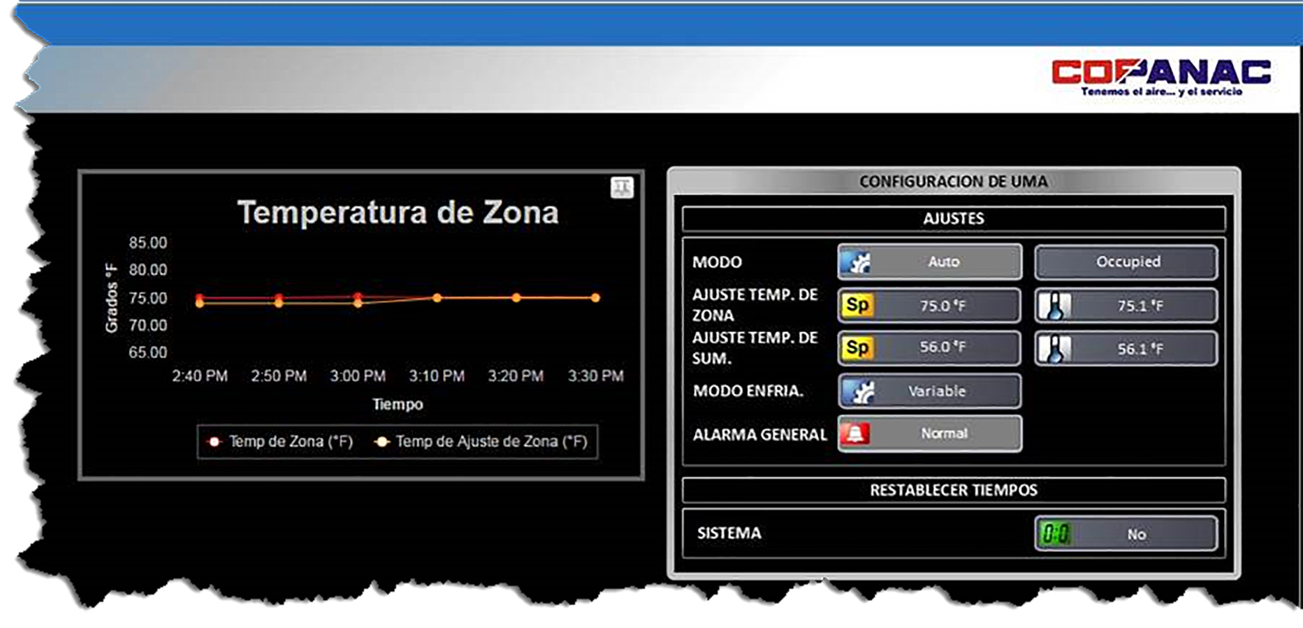
Figure 3: PI control accuracy displayed on System Group (Courtesy of COPANAC S.A.).

Derivative Rate (Deriv.)

When utilized, the derivative rate is tuned in minutes (0.00–2.00) and applies an immediate response to an anticipated future error. Improper use or tuning of a derivative rate can amplify noise, or oscillation, in the process. Proper derivative tuning often requires some trial and error over time.

1. Start with a small derivative rate.

2. The initial derivative rate can again be determined analogously or parametrically. In the absence of analogous or parametric data, consider 0.25 minutes.

3. Observe the response of the control loop through an input or setpoint change (disturbance). Be sure to provide adequate time to evaluate the responsiveness of the loop before making changes.

4. Following an input or setpoint change (disturbance), does the control loop hunt?

5. If the control loop does not hunt following a disturbance, increase the derivative rate by 0.25. Return to step 3.

6. If the control loop hunts following a disturbance, decrease the derivative rate by 50% of the last change. For instance, if the last change was an increase from 0.75 to 1.00, and the loop is now cycling, decrease the derivative rate to 0.88 (e.g., 1.00 - 0.75 = 0.25; 0.25 / 2 = 0.125; 1.00 – 0.12 = 0.88).

7. Observe the response of the control loop. Be sure to provide adequate time to evaluate the responsiveness of the loop before making changes.

8. Following a change in input or setpoint (disturbance), does the control loop hunt? If so, return to step 6.

9. Eventually the loop will provide an output that is appropriate to eliminate error without introducing process instability, excessive overshoot, and hunting.

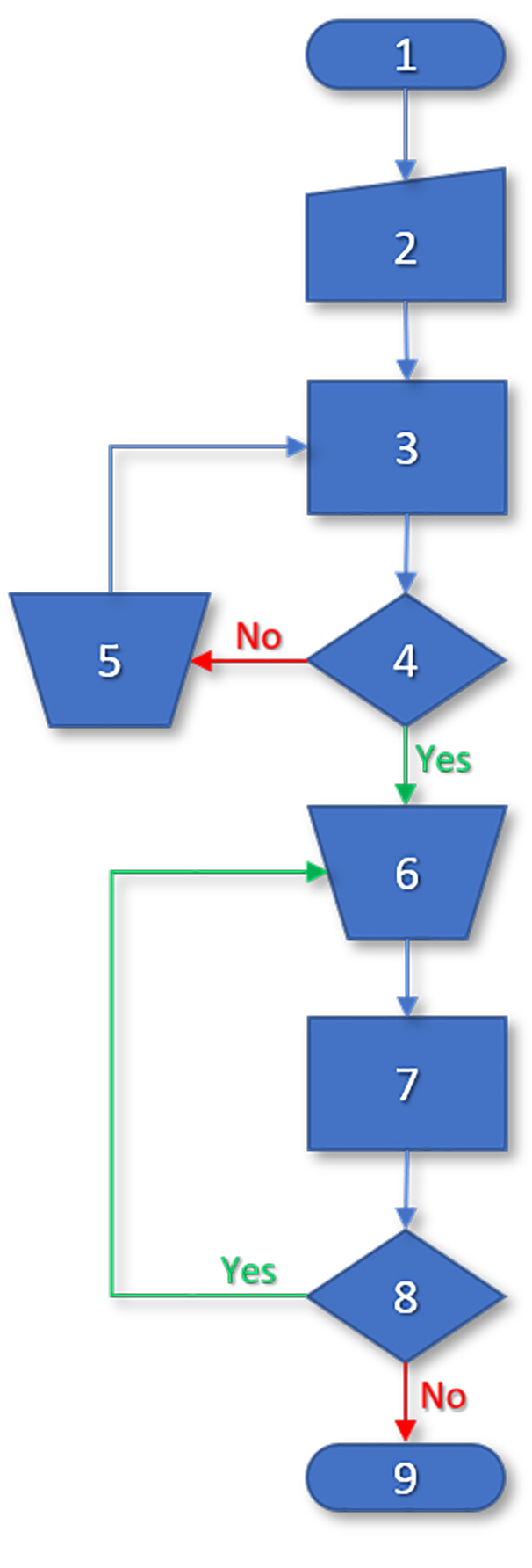
Figure 4: Derivative rate tuning process flowchart.

Bias

Bias is a constant offset. In stable processes, bias can be used to eliminate consistent offset; however, this is a less common use. Bias is not recommended as a replacement for an integral reset in variable systems. In dynamic processes, bias is commonly used to represent the continuous correction that is required to maintain process variables like pressure or flow. In these applications, the input cannot be maintained at the setpoint if the output is allowed to be reduced to zero.

Bias is most often configured and tuned as a constant like proportional, integral, and derivative. The most effective way to tune bias to a specific system is through observation of stable operation.

1. Begin with a neutral bias.

2. The initial bias can be determined analogously or parametrically. In the absence of analogous or parametric data, consider 40–50 percent.

3. Use a trend log to observe the response of the control loop over several hours or days of stable operation.

4. Identify the output that is most common or most consistent when the input is steadily maintained at or near the setpoint. If the initial bias is significantly incorrect, this will be the value to which the loop most often corrects, possibly with oscillation. Adjust the bias to this value.

5. Use a trend log to observe the response of the control loop again over several hours or days of stable operation.

6. Identify the output that is most common or most consistent when the input is steadily maintained at or near the setpoint. If it is different than the presently configured bias, adjust the bias to be halfway between the presently configured bias and the most consistent value. For example, if the present bias is 40 percent and the output when the input is steadily maintained is 46 percent, then modify the bias to 43 percent.

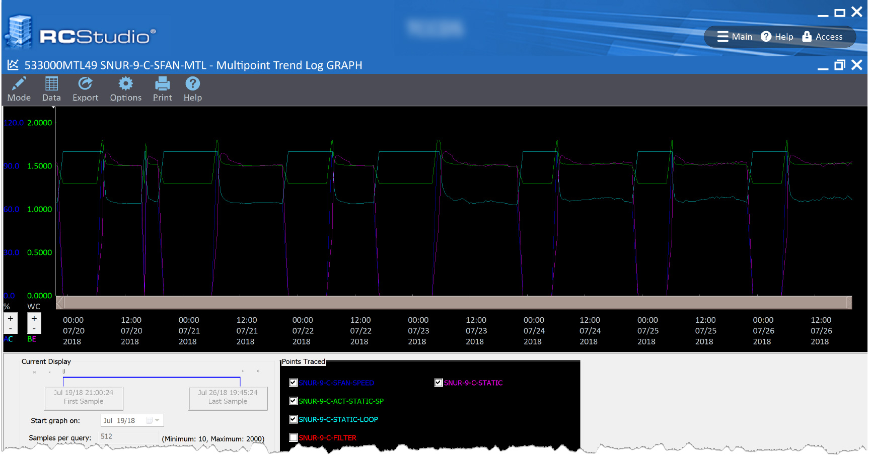
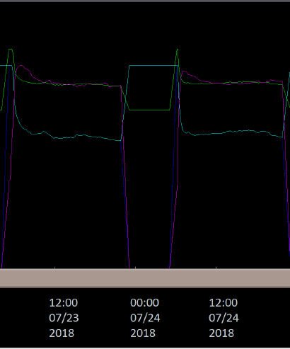
Some application engineers programmatically tune the bias continuously. One method is to allow a control loop to stabilize, and then slowly ramp the bias to match the output. This technique empowers the system to indirectly respond to changes in the process. While this method could result in some instability in rapidly changing processes, it has proven very effective in processes like duct static pressure control in variable air volume applications. Using this technique, with a simple, properly tuned PI loop and dynamic bias, Reliable Controls Authorized Dealers consistently deliver static pressure control with an average deviation from setpoint (error) of ≤ 0.04 inwc (10 Pa).

Figure 5: Trend log demonstrating stable PI loop control with dynamic bias (Courtesy of Environmatic Systems Inc.).

Deadband

Deadband is an optional term which can be helpful in reducing small amplitude hunting above and below the setpoint - sometimes called “dithering”. Because the deadband pauses correction around the setpoint, not only can it impact control precision, but it can directly impact the performance of the proportional band and the integral reset. The magnitude of the deadband is effectively added to the proportional band. Care must be taken when configuring a deadband to prevent the value from interfering with proper control.

When implementing and tuning deadband some trial and error over time can be required.

1. Begin with a small deadband.

2. The initial deadband can be determined analogously or parametrically. In the absence of analogous or parametric data, consider a deviation that would not require correction without impacting the process (e.g., perhaps 0.25-0.5˚).

3. Use a trend log to observe the response of the control loop over several hours or days of stable operation. Is the response of the process satisfactory? Is the offset satisfactory? Does the process hunt?

4. If the process performance and offset are satisfactory, and the process does not hunt, consider increasing the deadband by 25 percent. If the process performance and offset are unsatisfactory, or the introduction of deadband causes the process to hunt, consider decreasing the deadband by 25 percent.

5. Use a trend log to observe the response of the control loop over several hours or days of stable operation. Is the response of the process satisfactory? Is the offset satisfactory? Does the process hunt?

6. If the process performance and offset are satisfactory, and the process does not hunt, consider increasing the deadband by 50 percent of the last change. If the process performance and offset are unsatisfactory, or the introduction of deadband causes the process to hunt, consider decreasing the deadband by 50 percent of the last change.

There is a fine line between a properly tuned control loop and an obsession. MACH-System™ control loops can be tuned easily, quickly, and accurately for a wide variety of applications. Know when to stop. In many cases, rough-tuning can happen in one session. After this initial tuning is complete, it is recommended to trend the input, setpoint, output, and loop in a multipoint trend log with a relatively small polling period: perhaps once per minute or per five minutes in the beginning. Walk away and do something else, return at the end of the day and evaluate the loop. Return at the end of the week, or the month, and evaluate the loops. Make minor adjustments as appropriate. In this way, leverage trend logs to monitor performance.

The process is not prohibitive. If not perfect, practice makes better. The only way to become effective at tuning control loops is by tuning control loops. There was a time when no one could tune a control loop. Ask for help. Improperly tuned control loops are inexcusable from automation professionals.

Lead the Way

A symphony orchestra is comprised of professional musicians. They can play their instruments without a conductor. However, a conductor is so much more than a breathing metronome. The conductor’s trained, critical ear and highly-refined expertise complements the musicians to create art. Like a conductor, a skilled-automation professional can use understanding, critical observation, and highly-refined expertise to synchronize mechanical systems into a concerted ensemble. Like the emotion expressed in the gesture of a conductor, a finely-tuned control loop is a cornerstone of being reliable people and technology.