


ASHRAE Guideline 36 for high-performance HVAC systems
ASHRAE Guideline 36 represents an important synergy between standard high-performance designs and standard control applications.


Imagine keeping warm over a campfire on a cool evening. You see the flickering fingers of fire. Hear the snap, crackle, pop. Smell the woodsmoke on the breeze. Eventually the flames will burn low, and people will grow uncomfortably cool. No need to worry, though: The fire can be revived and the heat it generates refueled by throwing another log on and stoking the embers.
This is a simple example of process control. The fire represents a dynamic system. As fire consumes the wood, less fuel is available, which in turn leads to the release of less heat and light. When the amount of heat released falls below the comfort level, or control point, some corrective action is needed to bring the process back to a desirable state. Adding fuel to the fire is a control response intended to restore the process to a controlled condition.
Maintaining a campfire is manual process control. While little consideration is given to the discipline of process management in the moment, it exhibits the basic principles of control loop theory—the principle used by facility automation systems to perform automatic control every day. The control loop is the means to maintaining stable control of a process.
A control loop is a method to maintain a process in a desired state or to maintain a process variable within set control points or at a desired setpoint. Control loops are primarily concerned with three basic tasks:
Understanding how a control loop works hinges on a few basic concepts.
The process variable is a dynamic value or condition that is measured and ultimately controlled as part of the process. The process variable is the input to a control loop. In the campfire example, the input to the control loop is temperature. In facility automation control loops, common process variables, or inputs, include temperature, pressure, and flow. In a typical comfort control application, space temperature is often a control loop input; space temperature is the value that is measured and controlled.
The control point is the desired value of the process variable or the setpoint. In the campfire example, the setpoint is the desirable comfort level. An automatic control loop manipulates a process to maintain the process variable, or input, within minimum and maximum control limits or at a desired control setpoint. In a typical comfort control application, space temperature is often maintained between heating (minimum) and cooling (maximum) control limits or at a space temperature setpoint.
The error of a control loop is the difference between the measured process variable and the control point or the deviation between the input and the setpoint. In a typical comfort control application, if the space temperature is 74°F, and the setpoint is 72°F, the error is +2°F (74 - 72 = +2). This represents positive error or a positive deviation. If the space temperature is 21°C with a setpoint of 22°C, the error is -1°C (21 - 22 = -1), resulting in a negative error.
The ultimate objective of a control loop is to eliminate error. This is achieved by manipulating the process in some way through a control response or some corrective action. This control response is the output of the control loop. In a typical comfort control application, the space temperature might be manipulated through the introduction of warm or cool air.
Control loops are generally categorized as open-loop or closed-loop. These terms describe their execution methodology.
In open-loop control, the control response is independent of the process value. Open-loop control is a process without feedback. The value of the input is not considered in the control response. For example, cooking using a kitchen timer ensures only that heat is applied for a prescribed amount of time and gives no consideration to the temperature of the food. For many years, in some traditional comfort control applications, heating hot water and chilled water temperatures were manipulated or reset based on the ambient temperature outside with no consideration to the temperature inside a building. The oven affects the food just as the boilers and chillers affect the occupants, but using open-loop control, neither the food nor the occupants influence the output.
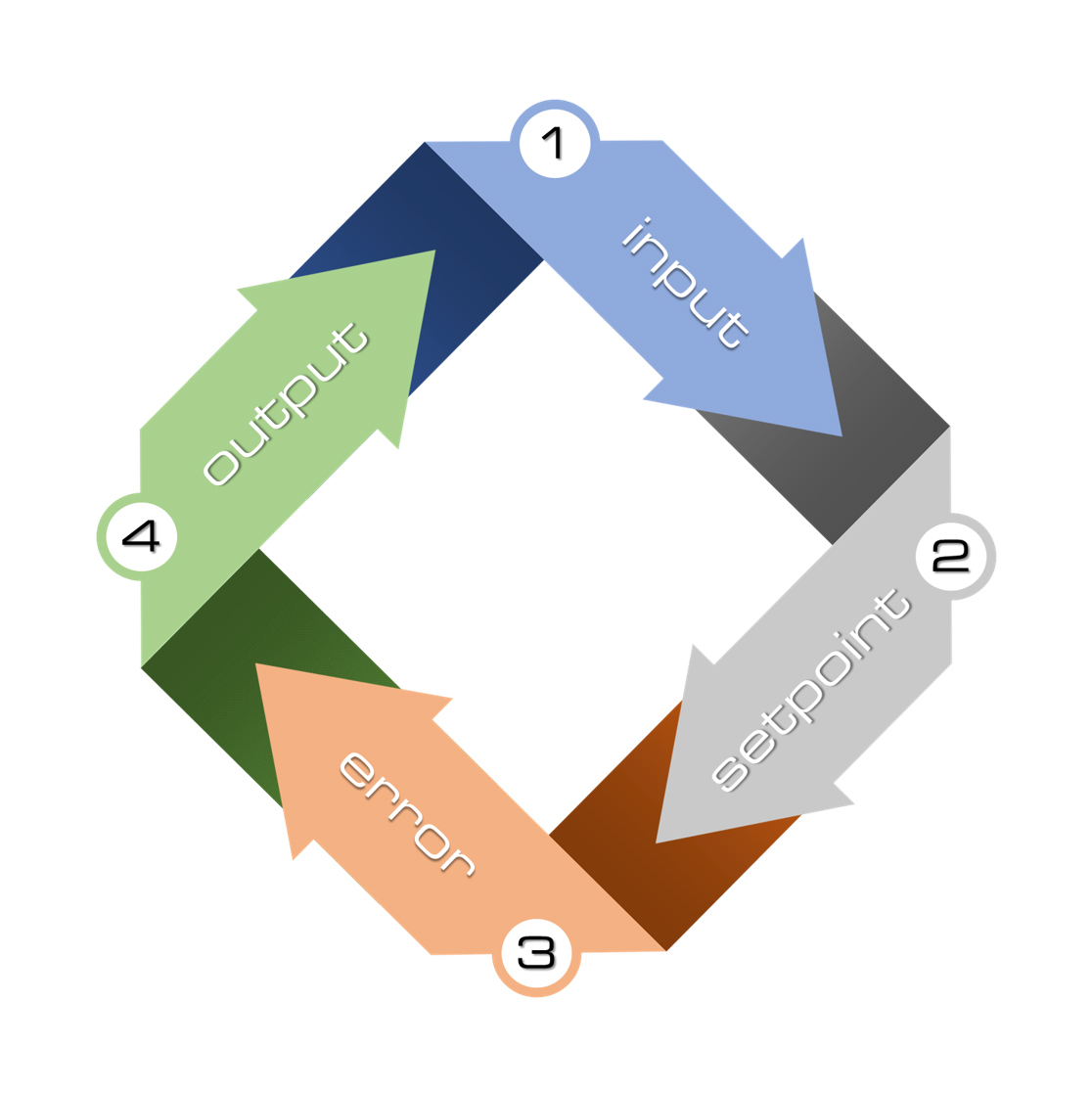
Proper control loop theory is primarily concerned with closed loops. In closed-loop control, also called feedback control, the process variable or input provides continuous feedback to the process, empowering the process to respond. This is a closed loop because each step in the process is connected to the next until the final step influences the first. All the steps interrelate in a continuous cycle or loop:
1. The input is measured.
2. The input is subtracted from the setpoint.
3. The resulting error is evaluated.
4. An appropriate output is determined.
5. The output influences the input.
The campfire represents closed-loop control. When proximity to the fire feels cool, more fuel is added. If too much wood is added, and the fire becomes uncomfortably warm, fuel can be removed. The comfort level, or input to the process, is constantly monitored and used to determine an appropriate control response or output. The control response influences the input, which is used to determine an appropriate response. Around and around the process goes.
In a typical comfort control application, the space temperature is continuously monitored, and the space temperature deviation from the setpoint is used to determine an appropriate response, perhaps modulating a valve or damper open or closed. This then influences the space temperature and subsequent correction.
Control loop theory is fundamental to industrial and facility control systems. Control loops are often embedded systems executed continuously by microprocessor-based controllers.
The Reliable Controls system uses a proportional integral derivative (PID) mathematical algorithm encapsulated in a standard BACnet control loop object.
A Reliable Controls system control loop evaluates several parameters to resolve a control response between 0 and 100 percent. Each parameter is configured independently to manage, and automatically evaluated to determine, the output value.
The action of a control loop is used to define how it responds to error.
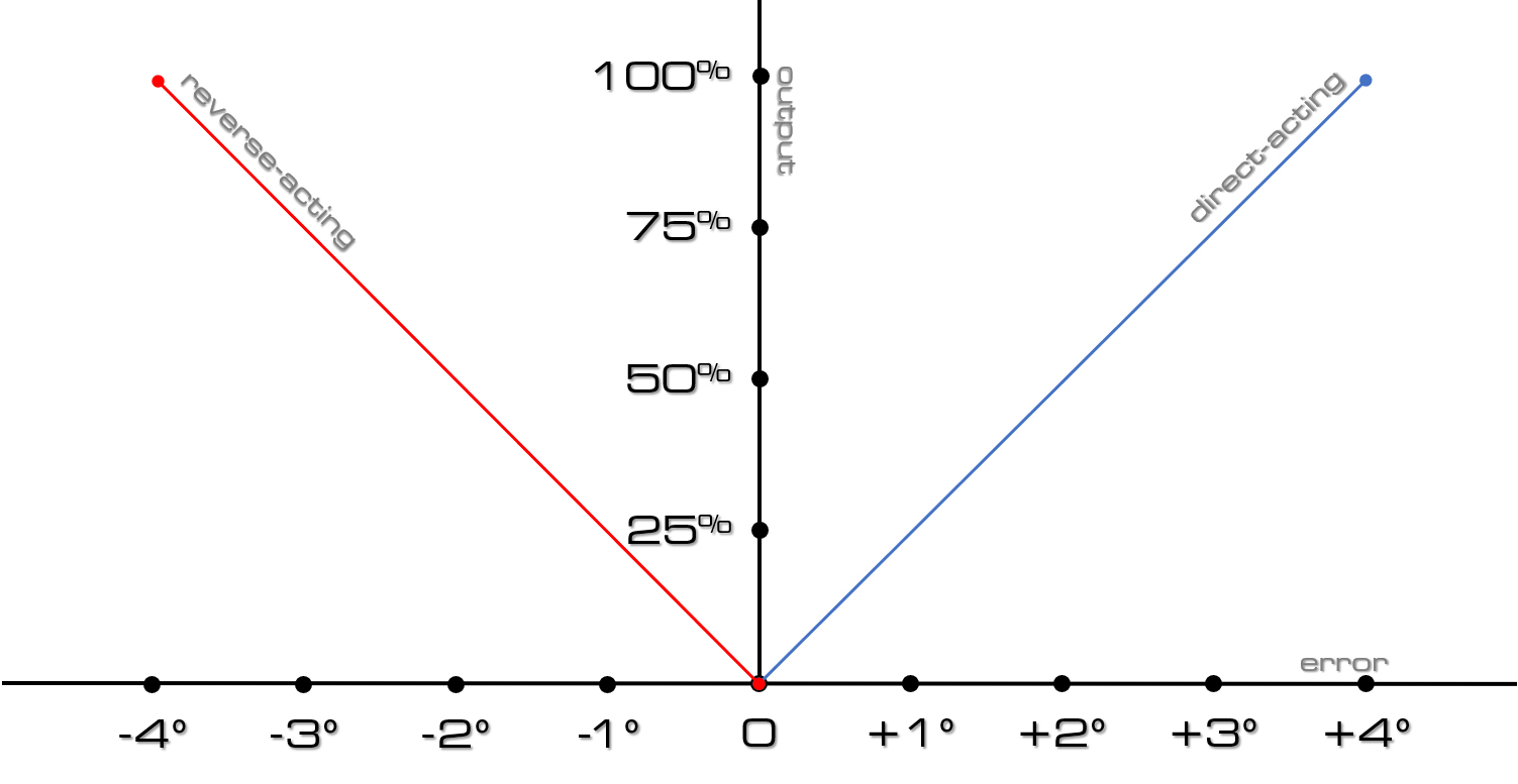
Direct-acting control loops provide positive correction in response to positive deviation and provide negative correction in response to negative deviation. As the value of the input increases, the output increases; when the value of the input decreases, the output decreases. Cooling applications are common examples of direct-acting control loops. As the temperature increases, more cooling must be provided, and as the temperature decreases, less cooling must be provided.
Reverse-acting control loops provide negative correction in response to positive deviation and provide positive correction in response to negative deviation. As the value of the input increases, the output decreases; when the value of the input decreases, the output increases. Heating applications are common examples of reverse-acting control loops. As the temperature increases, less heating must be provided, and as the temperature decreases, more heating must be provided.
A proportional control loop term is used to determine a control response based on error. The output is calculated in direct proportion to the deviation of the input from the setpoint. Greater deviation results in greater correction; less deviation results in less correction. A proportional term can be used as a standalone control loop (P loop), where it is often referred to as proportional control. It is also one corrective term of proportional integral (PI) and proportional integral derivative (PID) control loops.
Direct-acting and reverse-acting control loop action relative to error.
A proportional band is the proportional controller constant that defines the amount of deviation required to drive the corrective element through its entire operational range—for example, to modulate a valve from 0 to 100 percent.
In Reliable Controls system control loops, the proportional band is expressed in the units of the input (°C, °F) and defines the amount of deviation that results in 100 percent correction.
The proportional corrective action (Op) is calculated as:
Op = A * 100/Pb * (I - S)
Where:
The total corrective action is automatically limited to between 0 and 100 percent.
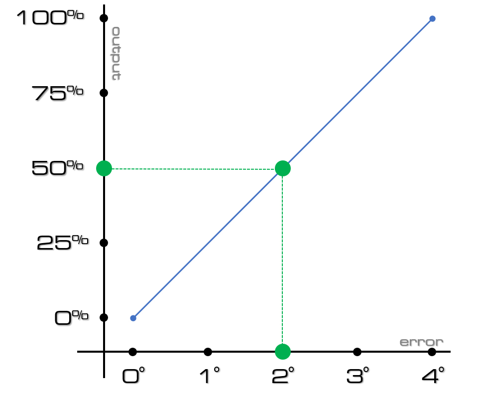
If a direct-acting proportional control loop is configured with a proportional band of 4°, the output linearly modulates from 0 to 100 percent in direct proportion to a deviation from setpoint of 0° to 4°.
Consider an example with a space temperature setpoint of 72°F. When the room temperature is 72°F, the deviation is 0°F, and the proportional output is 0 percent. When the room temperature is 74°F, the deviation is 2°F, and the proportional output is 50 percent. When the room temperature is ≥76°F, the deviation is ≥4°F, and the proportional output is 100 percent.
Proportional output example with a 4° proportional band.
A proportional control response requires a deviation. Remember, zero deviation results in zero proportional correction. When the deviation is stable, the correction remains constant. For example, imagine a process has a chilled water valve open 50 percent, and this corrective action is sufficient to maintain a 2° error or deviation. If the input does not change, the deviation does not change, which means the proportional output does not change. While this is stable control, it also represents a persistent 2° offset, or error, over time. Proportional control does not attempt to eliminate this offset. In some applications, minor sustained offset is acceptable. In applications where a persistent offset is unacceptable, an additional corrective term such as integral is added to the control loop.
An integral control loop term determines corrective action based on offset, or error, over time. If the duration and magnitude of the offset are short, the integral correction is small. As the duration or magnitude of the offset increases, so too does the accumulated integral correction. Integral correction is accumulated until there is no deviation. Integral can be used as a standalone control loop (I loop), where it is sometimes referred to as reset control, or used in floating control applications. It is also one corrective term of PI and PID control loops.
The response of an integral controller is adjusted by changing the integral action time or reset time.
In Reliable Controls system control loops, to set the integral reset, specify the number times per minute or per hour corrective action is accumulated.
The integral corrective action (Oi) is calculated as:
Oi = Oi + A * R * t 60 * (I - S)
Where:
The Oi is then adjusted such that the total corrective action is limited between 0 and 100 percent.
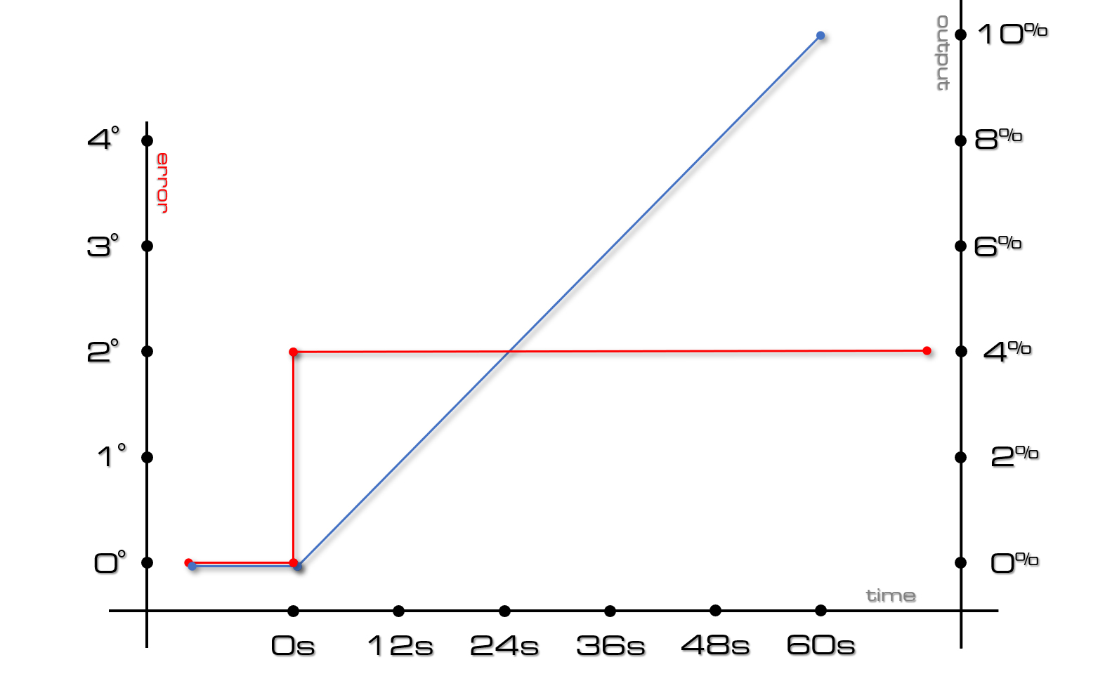
A corrective action equal to the magnitude of the error is added to or subtracted from the accumulated integral correction over time. This means a 2˚ error results in a correction of 2 percent, a 20˚ error results in a correction of 20 percent, and 0.2˚ error results in a correction of 0.2 percent. This correction is added to the accumulated integral correction based on the integral reset term. If the integral reset term is configured for five times per minute, the integral correction accumulates at a rate of once every 12 seconds (60 seconds in a minute/5 times per minute = 12 seconds).
With a stable error of 2˚ and an integral reset term of five times per minute, an integral correction of 2 percent is accumulated every 12 seconds:
Integral correction as a product of time over 60 seconds (2˚ error, five times per minute integral term).
Integral correction accumulates until there is no deviation. The accumulated integral correction is not reset to zero when the input reaches the setpoint. Some overshoot, correcting the process variable beyond the setpoint, is required to step down the accumulated integral correction. For example, in a direct-acting cooling application, the room temperature is likely to spend some time below the setpoint, resulting in negative offset, so the integral correction can be subtracted incrementally until it reaches zero.
For this reason, integral and proportional control are complementary. When used cooperatively in a PI loop, the integral correction can overcome the persistent offset common in proportional-only control, and the proportional correction can buffer the overshoot that an integral-only control loop could create.
A risk of improper integral control is integral wind-up. This is an undesirable situation where a large accumulation of integral correction occurs due to excessive offset, or error over time. Due to this excessive offset, an integral term could continue to correct, drastically overshooting the corrective action until the error is unwound. In other words, a commensurate amount of time must pass for the corrective action to return to normal. For example, a direct-acting cooling loop could accumulate integral correction for an entire weekend while the space is unoccupied, and the mechanical equipment is idle. Integral correction that was allowed to accumulate for 48 hours might take 48 hours to unwind or for the integral term to return to zero. To prevent drastic and unwanted integral wind-up, the integral term of all Reliable Controls system control loops is limited to between 0 and 100 percent.
Derivative is a control loop term that determines corrective action based on the rate of change of the error. If the process variable, or input, is changing, the derivative control loop term provides corrective action. When the input stops changing, regardless of the error or offset, the derivative corrective action is zero. A derivative term can be an anticipator to counteract change when very little error is acceptable and the corrective action, or output, may have an immediate and substantive effect on the process variable, or input. When used, derivative is often combined with another control loop method and is one term of PID control loops.
In Reliable Controls system control loops, the derivative is expressed in units of minutes, from 0.00 to 2.00 minutes, with a higher value resulting in a larger output to oppose the changing input.
The derivative corrective action (Od) is calculated as:
Od = A * D((I – S) – (It – 1 – St – 1)) / t
Where:
The nature of the derivative term can make it difficult to properly tune and is inappropriate for many comfort control applications where control responses seldom have an immediate and substantive effect on the process variable.
Control loops are fundamental to facility automation, and it can be easy to take the underlying theory for granted. But beware: Complacency, ignorance of proper process control technique, or the perception that control loops are magic are all equally likely to result in cold campfires and poorly performing buildings. Providing solutions that are better by design requires the best effort of control professionals throughout the Reliable Controls Authorized Dealer network.

ASHRAE Guideline 36 represents an important synergy between standard high-performance designs and standard control applications.

Data can present both an opportunity and obstacle to optimizing energy-consuming systems. How do you turn insights into action?

Explore how our technology automates complex enterprise portfolios.

Find out how APIs empower you to do more with your building with less effort.

We recently marked the sale of our millionth controller, a major milestone made even more meaningful thanks to the people who helped make it possible.

Learn how our building automation systems are designed to support you.
Here’s how we actively work to counter planned obsolescence with every product we make.

The MACH-ProLight is ideally positioned to implement advanced and adaptive lighting control strategies in new and existing facilities alike.